섹션 9. 서포트 벡터 회귀 (SVR, Support Vector Regression)

● URL : https://colab.research.google.com/drive/1YBZtRHrYPXoGHDxDHaQujgNpLtpHJVVq#scrollTo=xfoa8OSORfHQ

 

● 앱실론 무신경 튜브

: 범위 안에서 발생하는 오류는 신경쓰지 않는다.

따라서 여유 공간을 제공한다.

 

● 특성 스케일링을 적용하지 않는 경우

1) 가변수

2) 종속 변수가 0, 1과 같은 이진 값을 가진 경우

(+) 훈련 세트와 테스트 세트로 분할 할 경우 분할 후에 특성 스케일링을 적용한다.

 

● 특징

SVR 모델에는 특성에 관련된 명시적인 종속 변수의 방정식이 없다.

그리고 각각의 특성에 곱하는 계수도 없다.

낮은 특성 값을 보상해서 높은 값을 취하지도 않는다.

 

※ 종속 변수가 다른 특성에 비해 큰 값을 갖는 경우에는 특성 스케일링을 적용하여 모든 특성과 종속 변수를 같은 범주로 맞춰야한다.

※ 특성 스케일링을 특성 행렬 x과 종속 행렬 y에 모두 적용해야한다.

 

Step 1. Importing the libraries

import numpy as np

import matplotlib.pyplot as plt

import pandas as pd

 

Step 2. Importing the dataset

dataset = pd.read_csv('Position_Salaries.csv')

X = dataset.iloc[:, 1:-1].values

y = dataset.iloc[:, -1].values

--------------------------------------------------------------------------------------------------------------------------------------------------------------------

X : 2차원 벡터

y : 1차원 벡터

--------------------------------------------------------------------------------------------------------------------------------------------------------------------

y = y.reshape(len(y),1)

--------------------------------------------------------------------------------------------------------------------------------------------------------------------

특성 스케일링(표준화)를 수행할 StandardScaler 클래스가 입력값으로 특수한 형식 요구 - y : 2차원 배열로 변환

--------------------------------------------------------------------------------------------------------------------------------------------------------------------

 

Step 3. Feature Scaling

from sklearn.preprocessing import StandardScaler

sc_X = StandardScaler()

sc_y = StandardScaler()

X = sc_X.fit_transform(X)

y = sc_y.fit_transform(y)

--------------------------------------------------------------------------------------------------------------------------------------------------------------------

특성 행렬 x, 종속 행렬 y 모두 특성 스케일링 적용해야함으로 2개의 StandardScaler 인스턴스 생성

--------------------------------------------------------------------------------------------------------------------------------------------------------------------

 

Step 4. Training the SVR model on the whole dataset

- kernel (종류 : 선형 커널, 비선형 커널, 가우시안 RBF 커널, 가우시안 커널, 방사 기저 함수 RBF 커널 등등)

from sklearn.svm import SVR

regressor = SVR(kernel = 'rbf')

regressor.fit(X, y)

 

Step 5. Predicting a new result

- inverse_transform : 역변환(역스케일링) 함수

sc_y.inverse_transform(regressor.predict(sc_X.transform([[6.5]])).reshape(-1,1))

--------------------------------------------------------------------------------------------------------------------------------------------------------------------

원래의 스케일에서 예측을 얻기 위해서 예측 전체에 역스케일링을 적용한다.

(1) regressor.predict(sc_X.transform([[6.5]])) : 스케일링

(2) sc_y.inverse_transform(...).reshape(-1,1) : 예측값을 원래 스케일로 역변환

※ 예측값은 종속변수(y)이므로 sc_y으로 역변환한다.

(3) .reshape(-1,1) : inverse_transform 함수 충족 위해 예측된 값의 형식 변경

--------------------------------------------------------------------------------------------------------------------------------------------------------------------

 

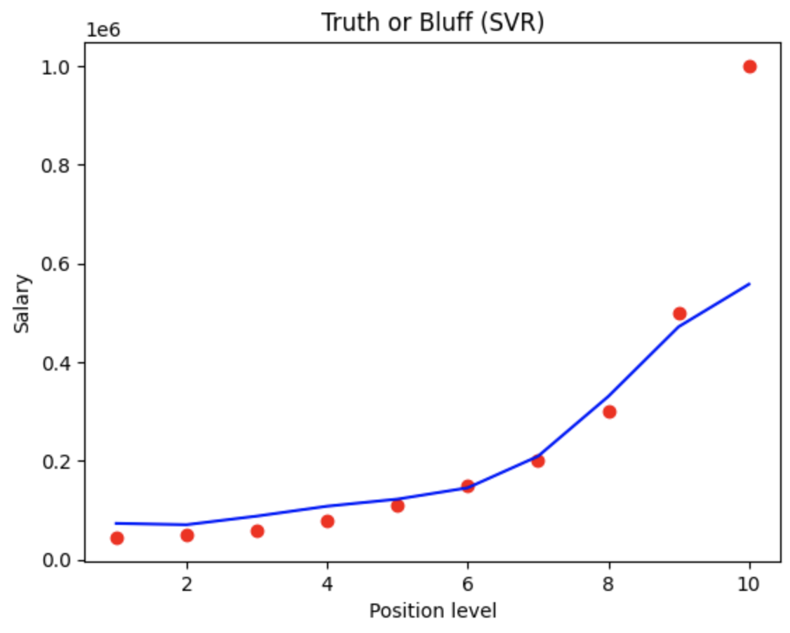
Step 6. Visualising the SVR results

plt.scatter(sc_X.inverse_transform(X), sc_y.inverse_transform(y), color = 'red')

plt.plot(sc_X.inverse_transform(X), sc_y.inverse_transform(regressor.predict(X).reshape(-1,1)), color = 'blue')

plt.title('Truth or Bluff (SVR)')

plt.xlabel('Position level')

plt.ylabel('Salary')

plt.show()

--------------------------------------------------------------------------------------------------------------------------------------------------------------------

(1) plt.scatter(sc_X.inverse_transform(X), sc_y.inverse_transform(y), ..) : 역변환 값

(2) plt.plot(sc_X.inverse_transform(X), sc_y.inverse_transform(regressor.predict(X).reshape(-1,1)), ..) : 역변환 값

--------------------------------------------------------------------------------------------------------------------------------------------------------------------

 

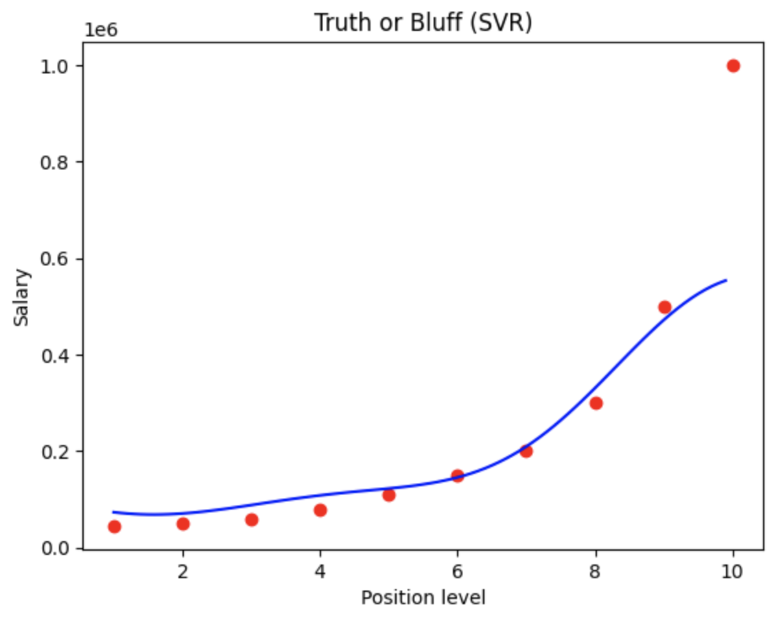
Step 7. Visualising the SVR results (for higher resolution and smoother curve)

X_grid = np.arange(min(sc_X.inverse_transform(X)), max(sc_X.inverse_transform(X)), 0.1)

X_grid = X_grid.reshape((len(X_grid), 1))

plt.scatter(sc_X.inverse_transform(X), sc_y.inverse_transform(y), color = 'red')

plt.plot(X_grid, sc_y.inverse_transform(regressor.predict(sc_X.transform(X_grid)).reshape(-1,1)), color = 'blue')

plt.title('Truth or Bluff (SVR)')

plt.xlabel('Position level')

plt.ylabel('Salary')

plt.show()